# NN Training
The learning block of the impulse design was configured as a Keras Classification block. In this block we have to configure the settings of a Neural Network (NN) and train the NN.
# NN settings
The neural network has several training settings and an architecture that can be configured. The training settings consist of a number of training cycles and a learning rate. The Number of training cycles means how much epochs a neural network has to be trained. An epoch is an instant in time chosen when something new starts, in the case of training a neural network an epoch denotes the start of a new training cycle. It could also be defined as "one pass over the entire dataset". The Learning rate will configure how fast the neural network learns. The learning rate is a factor that decides how big or small the update of a node its weight will be. If the network overfits quickly, then lower the learning rate. The default number of training cycles configured in Edge Impulse is 30, and the default learning rate is 0.0005.
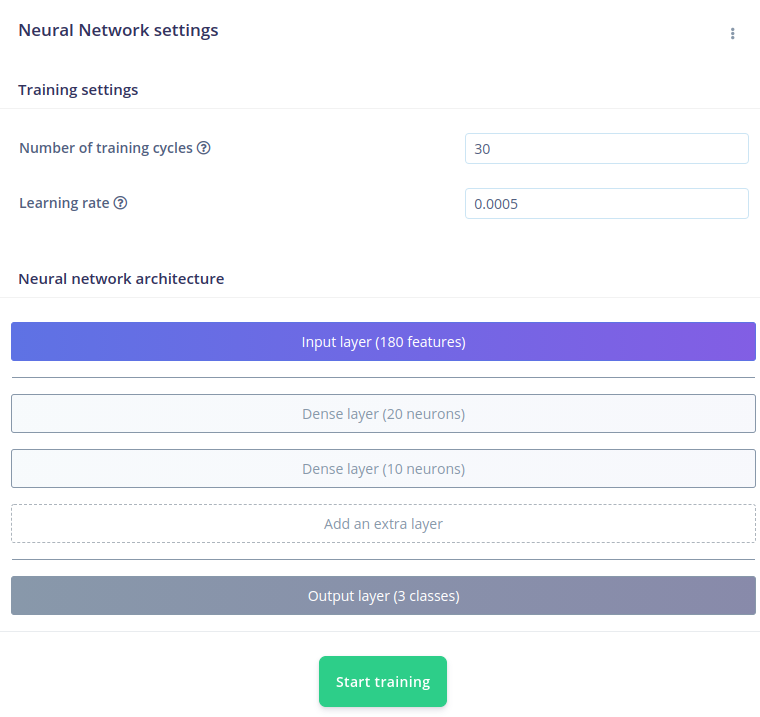
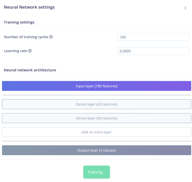
Because we have a quite small data set we are going to change the number of training cycles to 100. The learning rate we will leave as-is.
Hyperparameters
The number of epochs and learning rate are a part of the hyperparameters of a neural network. You don't have to follow the numbers of this workshop and can change them to achieve better (or worse) training results.
# NN architecture
Next in the NN settings is the NN architecture where we configure the layout of the AI model. As in the introduction and "hello world"-example, we have to configure inputs, outputs and some layers in between. In this case our number of inputs is configured by the feature generation step. We can see that the number of inputs is 180 features. How do we get this number?
- One window was configured as 600 ms.
- Our sampling frequency is 100 Hz.
- This would mean 60 samples per window.
- We have three axes with inputs (accX, accY and accZ).
- We are performing no special feature extraction, the signal processing block its output is the raw data.
- 60 samples x 3 axes = 180 features
The number of output classes is fixed to 3 and are the three labels we configured during data acquisition.
The layers in between are pre-configured and the default is two dense (or fully connected) layers with 20 and 10 neurons (or nodes) respectively. We can train the network with these settings, but it would underperform. In this example we change the number of neurons to 60 and 30 respectively. This can be done by hovering over the layer and clicking the "edit" button (with pencil).

Dense/FC layer
A dense or Fully Connected layer is a layer of nodes where all the inputs are connected to all the nodes and all the nodes will be connected with the next layer. So every node can be influenced by all the inputs.
If desired, one can remove or add extra layers to the network architecture. Different types of layers are possible but are not discussed further in this workshop. More details about the layers used in Edge Impulse and all other configurable layers can be found in the Keras Layers API (opens new window).
# NN training
All configurations are set to start training the network. When pressing Start training, the settings and parameters are sent towards a training node of the Edge Impulse cloud servers. In the Training output window you can follow the progress of your job. You will see the number of epochs passing by and see the evolution of the accuracy and loss values. The definitions of these parameters is:
- loss: The value that a neural network is trying to minimize. It's the distance between the ground truth and the predictions. In order to minimize this value or distance, the neural network learns by adjusting weighs and biases so that it reduces the loss.
- accuracy: The percentage of instances that are correctly classified. In our cases this denotes how many windows were correctly classified.
- val_loss: The loss for the testing or validation dataset.
- val_accuracy: The accuracy for the testing or validation dataset.
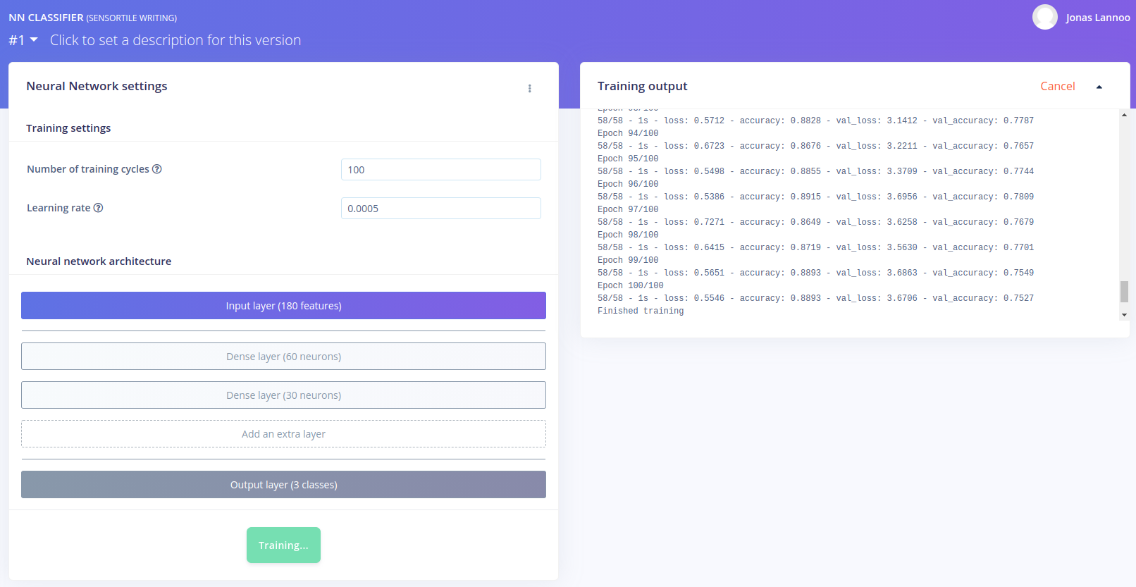
When the training is done, a summary is given of the training results. They are discussed in the next section.
# NN results
The training results consists out of five parts. Every part is explained in detail using the two figures below.
- Model selection
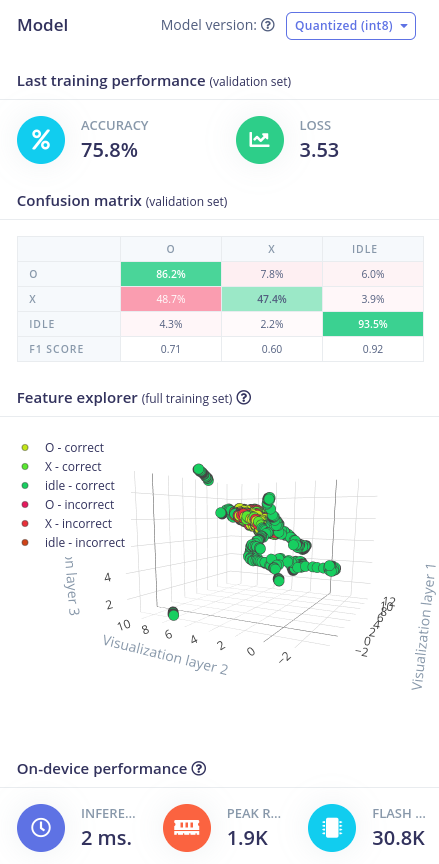
- Last training performance (on the validation data set)
- Confusion matrix (on the validation data set)
- Feature explorer
- On-device performance (of the NN only on your specified device)
# Model version
At the top of the "model results"-window we can select two versions:
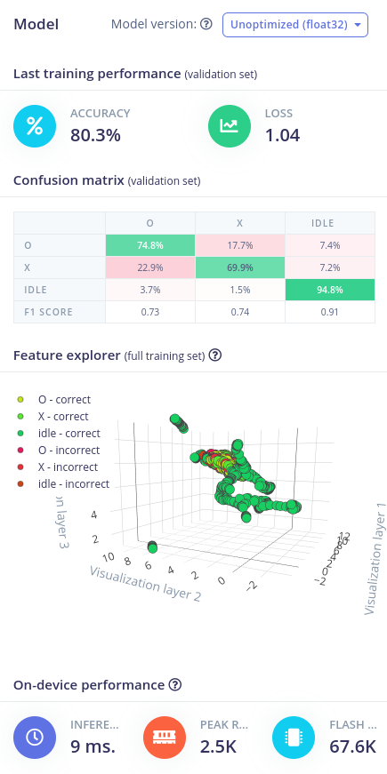
- Unoptimised (float32): This model is not optimized (or quantised) to run on a microcontroller and will use more memory space and longer inference time.
- Optimised (int8): This model is optimized (and thus quantised from 32-bit floating point to 8-bit integer values) to run on a microcontroller and will use less memory space and less inference time.
# Last training performance
The last training performance can be indicated with two metrics, the accuracy and the loss. Both are shown here on the testing or validation dataset (so not the result of the training itself). The definition of accuracy and loss has been given previously.
We can see that the accuracy and loss are worse for the microcontroller-optimized (quantised) model. Worse accuracy means lower, worse loss means higher. This is due to the fact that we convert the weights in the nodes of the network from a floating point value (allmost all possible numbers) to 8-bit integers (0-255).
Dynamic range
The effect of the quantisation step can be improved by have a lower dynamic range of the acquired data. For example, most windows have sample values between -5 and +5. There is one window which has an outlayer of +20 because of noise or abrupt movements. When converting the data for training, all values are normalised. This means that they are scaled relative to the maximum value. In this way we will lose precision when quantising the weights.
# Confusion matrix
The confusion matrix shows the performance of the network on the validation dataset for each type of input (window) and its calculated output. The percentage of each classification is given through this matrix. For example in the unoptimised case, the percentage of written 'O's that were actually recognised as 'O's is 74.8%. The other 25.2% of 'O's were classified as 'X' or 'idle' and their percentages can be found in the rest of that row. The same frame of thought can be done for the other rows. Edge Impulse will show how good the percentages are with colors.
The F1 score is another metric on how good the network classified the given inputs to its outputs. More information on the F1 score can be found here (opens new window).
We can see that the confusion matrix is worse for the quantised model, again for the same reason as the worsening of the training performance. We can also see that the network has more difficulty in recognising and 'X' as an 'X' and that it classifies it for almost 50% of the time as an 'O'. The network has no problems classifying the idle state of the pencil.
# Feature explorer
The feature explorer will give us a visualisation of the classified windows in a 3D view. The different colors are represented by the three labels (X, O and idle) and if they were correctly or incorrectly classified. By clicking on one we can see the sample in detail and see what features were used to classifiy this window. In this way you can debug your data set and evaluate the features.
# On-device performance
Lastly, the on-device performance is estimated by Edge Impulse according to your configured device (in the Dashboard). In this case, it is done for a Cortex-M4F 80 MHz microcontroller. The performance uses three metrices:
- Inferencing time: This is the time that it will take on the microcontroller to classify one input using the neural network.
- Peak RAM usage: This is the amount of RAM that will be used by the system.
- Flash usage: This is the amount of Flash memory that will be used by the system.
It is important to check these values. Depending on the application, the inferencing time should be within the imposed time frame for classifying an input window. Additionally, the RAM and flash memory should fit on your device under test.
# Next steps
Now that we have a trained network, we can classify new real-world inputs and see how well our neural network performs! Please go over to the next chapter where we start with live classification of new data.
